반응형
시계열 데이터 - 시간에 관련된, 시간을 표시할 수 있는 데이터
판다스에서 시계열 데이터 표현에 자주 이용되는 두 가지 유형이다.
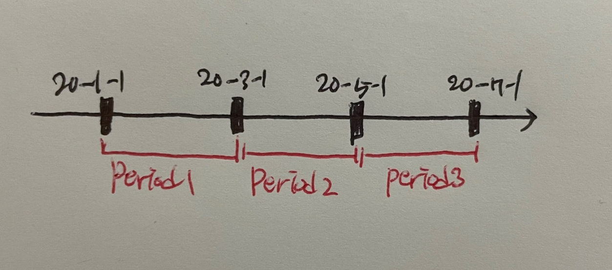
1. 두 시점 사이의 기간을 나타내는 Period
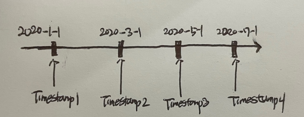
2. 특정한 시점을 기록하는 Timestamp
### 시계열 객체로 변환 ###
|
1
2
3
|
# 많은 날짜, 시간 데이터는 별도의 시간 자료형으로 기록된 것이
# 아니라 문자열 또는 숫자형으로 기록된 경우가 많다.
# 따라서 이러한 데이터를 시계열 객체로 변환해 주어야 한다.
|
cs |
## 문자열을 Timestamp로 변환 ##
|
1
2
3
4
5
6
7
8
9
10
11
12
13
14
15
16
17
18
19
20
21
22
23
24
25
26
27
28
29
30
31
32
33
34
35
36
37
38
39
40
41
42
43
44
45
46
47
48
49
50
|
## 문자열을 Timestamp로 변환 ##
# to_datetime() 함수를 사용해서 다른 자료형을 datetime64 자료형으로 변환 #
df = pd.read_csv("C:/Users/ZenBook/Desktop/code/sample/part5/stock-data.csv")
# 날짜 데이터가 포함된 csv파일 불러오기 (주식 시장에서 거래되는 거래 데이터)
print(df.info())
'''
<class 'pandas.core.frame.DataFrame'>
RangeIndex: 20 entries, 0 to 19
Data columns (total 6 columns):
# Column Non-Null Count Dtype
--- ------ -------------- -----
0 Date 20 non-null object
1 Close 20 non-null int64
2 Start 20 non-null int64
3 High 20 non-null int64
4 Low 20 non-null int64
5 Volume 20 non-null int64
dtypes: int64(5), object(1)
memory usage: 1.1+ KB
'''
# Data 자료는 날짜를 표시하는 데이터인데 현재 문자열(object)자료형을 저장되어있다.
df['new_Date'] = pd.to_datetime(df['Date'])
# 'Date' 열의 데이터를 시계열 데이터(datetime64) 자료형으로 변환하고 새로운 열에 저장
print(df.info())
'''
6 new_Date 20 non-null datetime64[ns]
'''
print(df['new_Date'][0])
'''
2018-07-02 00:00:00
'''
df.set_index('new_Date', inplace= True)
df.drop('Date', axis= 1, inplace= True)
# new_Date 열을 행 인덱스로 지정하고 Date 열을 삭제한다.
# 시계열 데이터를 행 인덱스로 지정함으로써 시간 순서에 맞게 데이터 분석이 쉬워진다.
print(df.head())
'''
Close Start High Low Volume
new_Date
2018-07-02 10100 10850 10900 10000 137977
2018-06-29 10700 10550 10900 9990 170253
2018-06-28 10400 10900 10950 10150 155769
2018-06-27 10900 10800 11050 10500 133548
2018-06-26 10800 10900 11000 10700 63039
'''
|
cs |
## Timestamp를 Period로 변환 ##
|
1
2
3
4
5
6
7
8
9
10
11
12
13
14
15
16
17
18
19
20
21
22
23
24
25
26
27
28
29
|
## Timestamp를 Period로 변환 ##
# to_period() 함수를 이용해서 일정한 기간을 나타내는 Period 객체로 변환 가능 #
dates = ['2019-07-08', '2000-04-22', '2000-10-31']
# 날짜를 나타내는 데이터 (문자열 자료형)
ts_dates = pd.to_datetime(dates)
# 문자열자료형을 Timestamp 객체로 변환
pr_day = ts_dates.to_period(freq='D')
# datetime64 자료형 -> period 자료형, freq='D' : 기준이 1일
print(pr_day)
'''
PeriodIndex(['2019-07-08', '2000-04-22', '2000-10-31'], dtype='period[D]')
'''
pr_month = ts_dates.to_period(freq='M')
# datetime64 자료형 -> period 자료형, freq='M' : 기준이 1달
print(pr_month)
'''
PeriodIndex(['2019-07', '2000-04', '2000-10'], dtype='period[M]')
'''
pr_year = ts_dates.to_period(freq='A')
# datetime64 자료형 -> period 자료형, freq='A' : 기준이 1년
print(pr_year)
'''
PeriodIndex(['2019', '2000', '2000'], dtype='period[A-DEC]')
'''
|
cs |
### 시계열 데이터 만들기 ###
## Timestamp 배열 만들기 ##
|
1
2
3
4
5
6
7
8
9
10
11
12
13
14
15
16
17
18
|
### 시계열 데이터 만들기 ###
## Timestamp 배열 만들기 ##
# date_range() 함수로 여러 개의 Timestamp가 들어 있는 배열 형태의 시계열 데이터 생성 #
ts_ms = pd.date_range(start='2020-01-01', # 2020-01-01을 시작해서 Timestamp 만듬
end = None, # 범위는 따로 정하지 않음
periods = 6, # Timestamp 6개 만듬
freq = 'MS', # 'M': 월, 'S': 시작일 ex)3M : 3달 간격
tz = 'Asia/Seoul') # 기준 시간 : 서울
# 2020-01-01 에 시작해서 한달 간격으로 Timestamp를 6개 만든다.
print(ts_ms)
'''
DatetimeIndex(['2020-01-01 00:00:00+09:00', '2020-02-01 00:00:00+09:00',
'2020-03-01 00:00:00+09:00', '2020-04-01 00:00:00+09:00',
'2020-05-01 00:00:00+09:00', '2020-06-01 00:00:00+09:00'],
dtype='datetime64[ns, Asia/Seoul]', freq='MS')
'''
|
cs |
## Period 배열 만들기 ##
|
1
2
3
4
5
6
7
8
9
10
11
12
13
|
## Period 배열 만들기 ##
pr_m = pd.period_range(start = '2020-01-01', # 2020-01-01을 시작으로 period 만듬
end = None, # 범위는 따로 정하지 않음
periods = 3, # period 3개 만듬
freq = '2H') # 기간의 길이 : 2시간
# 2020-01-01을 시작으로 기간이 2시간인 period 3개 만든다.
print(pr_m)
'''
PeriodIndex(['2020-01-01 00:00', '2020-01-01 02:00', '2020-01-01 04:00'], dtype='period[2H]')
'''
print(df.head())
|
cs |
### 시계열 데이터 활용 ###
## 날짜 데이터 분리 ##
|
1
2
3
4
5
6
7
8
9
10
11
12
13
14
15
16
17
18
19
20
21
22
23
24
25
26
|
### 시계열 데이터 활용 ###
## 날짜 데이터 분리 ##
# 날짜 데이터를 년 - 월 - 일 각각으로 분리한다 #
# dt.year, dt.month, dt.day 사용 #
df = pd.read_csv("C:/Users/ZenBook/Desktop/code/sample/part5/stock-data.csv")
# 날짜 데이터가 포함된 csv파일 불러오기 (주식 시장에서 거래되는 거래 데이터)
df['new_Date'] = pd.to_datetime(df['Date'])
# 'Date' 열의 데이터를 시계열 데이터(datetime64) 자료형으로 변환하고 새로운 열에 저장
df['Year'] = df['new_Date'].dt.year
df['Month'] = df['new_Date'].dt.month
df['Day'] = df['new_Date'].dt.day
# Timestamp 객체로 변환된 데이터 'new-Date를 년, 월, 일로 구분해서 데이터프레임에 추가한다.
print(df.head())
'''
Date Close Start High Low Volume new_Date Year Month Day
0 2018-07-02 10100 10850 10900 10000 137977 2018-07-02 2018 7 2
1 2018-06-29 10700 10550 10900 9990 170253 2018-06-29 2018 6 29
2 2018-06-28 10400 10900 10950 10150 155769 2018-06-28 2018 6 28
3 2018-06-27 10900 10800 11050 10500 133548 2018-06-27 2018 6 27
4 2018-06-26 10800 10900 11000 10700 63039 2018-06-26 2018 6 26
'''
|
cs |
반응형
'Pandas' 카테고리의 다른 글
| 필터링 (0) | 2022.11.09 |
|---|---|
| 함수 매핑 (1) | 2022.11.09 |
| 데이터 전처리 - 정규화 (0) | 2022.11.08 |
| 데이터 전처리 - 범주형(category) 데이터 처리 (0) | 2022.11.08 |
| 데이터 전처리 - 데이터 표준화 (0) | 2022.11.08 |